Understanding and Implementing CycleGAN in TensorFlow
Introduction
Transferring characteristics from one image to another is an exciting proposition. How cool would it be if you could take a photo and convert it into the style of Van Gogh or Picasso!
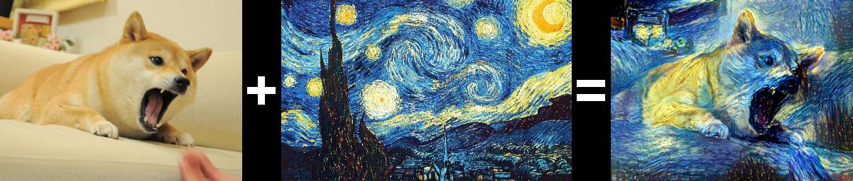
Starry Doge
Or maybe you want to put a smile on Agent 42's face with the virally popular Faceapp

A happy hitman
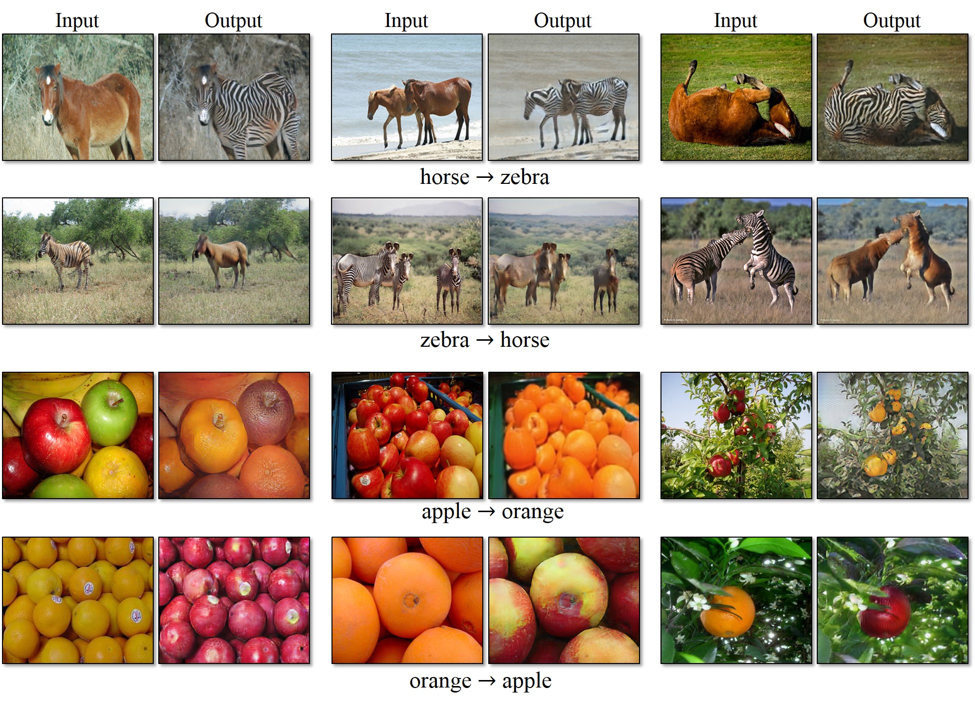
These are examples of cross domain image transfer - we want to take an image from an input domain $D_i$ and then transform it into an image of target domain $D_t$ without necessarily having a one-to-one mapping between images from input to target domain in the training set. Relaxation of having one-to-one mapping makes this formulation quite powerful - the same method could be used to tackle a variety of problems by varying the input-output domain pairs - performing artistic style transfer, adding bokeh effect to phone camera photos, creating outline maps from satellite images or convert horses to zebras and vice versa!! This is achieved by a type of generative model, specifically a Generative Adversarial Network dubbed CycleGAN by the authors of this paper. Here are some examples of what CycleGAN can do.
We are not going to go look at GANs from scratch, check out this simplified tutorial to get a hang of it. This workshop video at NIPS 2016 by Ian Goodfellow (the guy behind the GANs) is also a great resource. What we will be doing in this post is look at how to implement a CycleGAN in Tensorflow.
The paper we are going to implement is titled "Unpaired Image-to-Image Translation using Cycle-Consistent Adversarial Networks". The title is quite a mouthful and it helps to look at each phrase individually before trying to understand the model all at once
Unpaired Image-to-Image Translation
Figure from the paper
As mentioned earlier, the CycleGAN works without paired examples of transformation from source to target domain. Recent methods such as Pix2Pix depend on the availaibilty of training examples where the same data is available in both domains. The power of CycleGAN lies in being able to learn such transformations without one-to-one mapping between training data in source and target domains. The need for a paired image in the target domain is eliminated by making a two-step transformation of source domain image - first by trying to map it to target domain and then back to the original image. Mapping the image to target domain is done using a generator network and the quality of this generated image is improved by pitching the generator against a discrimintor (as described below)
Adversarial Networks
We have a generator network and discriminator network playing against each other. The generator tries to produce samples from the desired distribution and the discriminator tries to predict if the sample is from the actual distribution or produced by the generator. The generator and discriminator are trained jointly. The effect this has is that eventually the generator learns to approximate the underlying distribution completely and the discriminator is left guessing randomly.Cycle-Consistent
The above adversarial method of training has a problem though. Quoting the authors of the original paper:Adversarial training can, in theory, learn mappings $G$ and $F$ that produce outputs identically distributed as target domains $Y$ and $X$ respectively. However, with large enough capacity, a network can map the same set of input images to any random permutation of images in the target domain, where any of the learned mappings can induce an output distribution that matches the target distribution. Thus, an adversarial loss alone cannot guarantee that the learned function can map an individual input $x_i$ to a desired output $y_i$.
To regularize the model, the authors introduce the constraint of cycle-consistency - if we transform from source distribution to target and then back again to source distribution, we should get samples from our source distribution.
Network Architecture
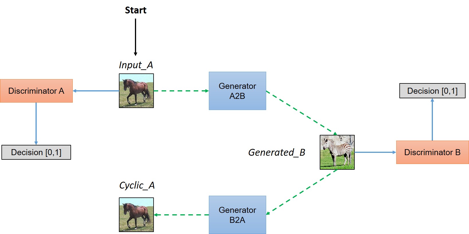
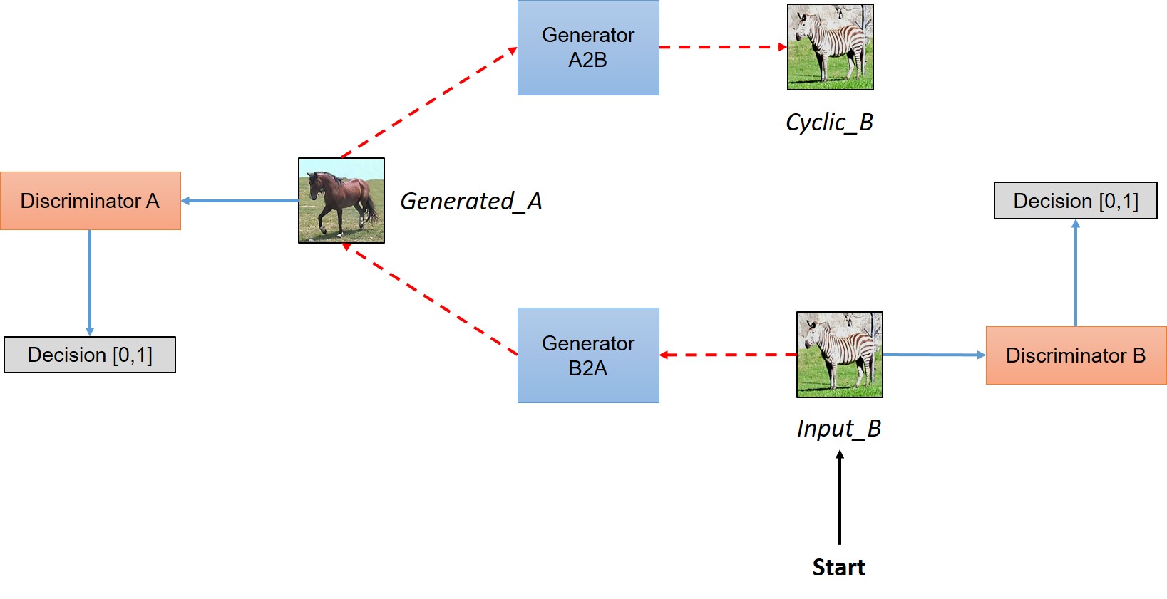
Simplified view of CycleGAN architecture
In a paired dataset, every image, say $img_A$, is manually mapped to some image, say $img_B$, in target domain, such that they share various features. Features that can be used to map an image $(img_A/img_B)$ to its correspondingly mapped counterpart $(img_B/img_A)$. Basically, pairing is done to make input and output share some common features. This mapping defines meaningful transformation of an image from one damain to another domain. So, when we have paired dataset, generator must take an input, say $input_A$, from domain $D_A$ and map this image to an output image, say $gen_B$, which must be close to its mapped counterpart. But we don't have this luxury in unpaired dataset, there is no pre-defined meaningful transformation that we can learn, so, we will create it. We need to make sure that there is some meaningful relation between input image and generated image. So, authors tried to enforce this by saying that Generator will map input image $(input_A)$ from domain $D_A$ to some image in target domain $D_B$, but to make sure that there is meaningful relation between these images, they must share some feature, features that can be used to map this output image back to input image, so there must be another generator that must be able to map back this output image back to original input. So, you can see this condition defining a meaningful mapping between $input_A$ and $gen_B$.
In a nutshell, the model works by taking an input image from domain $D_A$ which is fed to our first generator $Generator_{A\rightarrow B}$ whose job is to transform a given image from domain $D_A$ to an image in target domain $D_B$. This new generated image is then fed to another generator $Generator_{B\rightarrow A}$ which converts it back into an image, $Cyclic_A$, from our original domain $D_A$ (think of autoencoders, except that our latent space is $D_t$). And as we discussed in above paragraph, this output image must be close to original input image to define a meaningful mapping that is absent in unpaired dataset.
As you can see in above figure, two inputs are fed into each discriminator(one is original image corresponding to that domain and other is the generated image via a generator) and the job of discriminator is to distinguish between them, so that discriminator is able to defy the adversary (in this case generator) and reject images generated by it. While the generator would like to make sure that these images get accepted by the discriminator, so it will try to generate images which are very close to original images in Class $D_B$. (In fact, the generator and discriminator are actually playing a game whose Nash equilibrium is achieved when the generator's distribution becomes same as the desired distribution)
Implementing CycleGAN in tensorflow is quite straightforward. The following sections explain the implementation of components of CycleGAN and the complete code can be found here.
Building the generator
High level structure of Generator can be viewed in the following image.
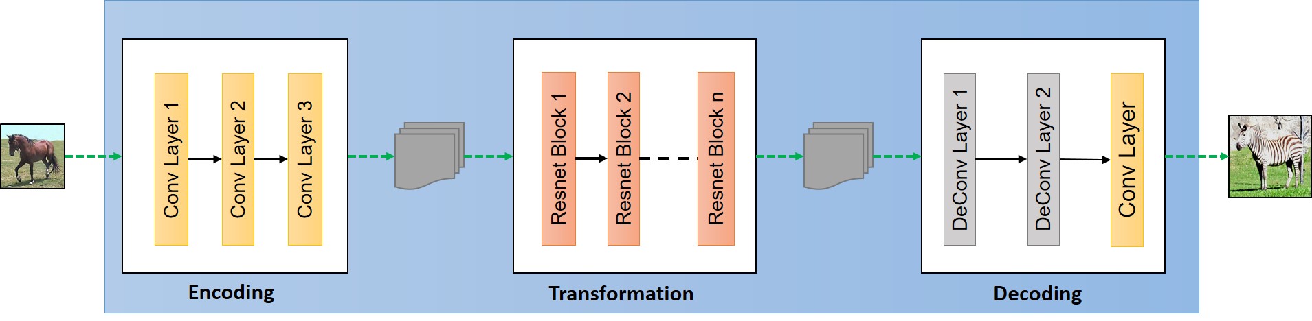
The generator have three components:
- Encoder
- Transformer
- Decoder
Following are the parameters we have used for the mode.
ngf = 32 # Number of filters in first layer of generator
ndf = 64 # Number of filters in first layer of discriminator
batch_size = 1 # batch_size
pool_size = 50 # pool_size
img_width = 256 # Imput image will of width 256
img_height = 256 # Input image will be of height 256
img_depth = 3 # RGB format
First three parameters are self explanatory and we will explain what pool_size means in the Generated Image Pool section.
Encoding:
For the purpose of simplicity, throughout the article we will assume that the input size is $[256, 256, 3]$. The first step is extracting the features from an image which is done a convolution network. To learn the basics about convolutional networks you can go through this very intuitive blog post by ujjwalkarn. As input a convolution network takes an image, size of filter window that we move over input image to extract out features and the stride size to decide how much we will move filter window after each step. So the first layer of encoding looks like this:
o_c1 = general_conv2d(input_gen,
                      num_features=ngf,
                      window_width=7,
                      window_height=7,
                      stride_width=1,
                      stride_height=1)
Here input_gen is the input image to the generator, num_features is the number of output features we extract out of the convolution layer, which can also be seen as number of different filters used to extract different features. window_width and window_height denote the width and heigth of filter window that we will move accross the input image to extract features and similarly stride_width and stride_height defines the shift of filter patch after each step. The output $o_{c_1}$ is a tensor of dimensions $[256, 256, 64]$ which is again passed through another convolution layer. Here, ngf = 64 as mentioned earlier. I have defined the general_conv2d function. We can add other layers like relu or batch normalization layer but we are skipping the details of these layers in this tutorial.
def general_conv2d(inputconv, o_d=64, f_h=7, f_w=7, s_h=1, s_w=1):
    with tf.variable_scope(name):
        conv = tf.contrib.layers.conv2d(inputconv, num_features, [window_width, window_height], [stride_width, stride_height],
                                        padding, activation_fn=None, weights_initializer=tf.truncated_normal_initializer(stddev=stddev),
                                        biases_initializer=tf.constant_initializer(0.0))
Further:
o_c2 = general_conv2d(o_c1, num_features=64*2, window_width=3, window_height=3, stride_width=2, stride_height=2)
# o_c2.shape = (128, 128, 128)

o_enc_A = general_conv2d(o_c2, num_features=64*4, window_width=3, window_height=3, stride_width=2, stride_height=2)
# o_enc_A.shape = (64, 64, 256)
Each convolution layer leads to extraction of progressively higher level features. It can also be seen as compressing an image into 256 features vectors of size 64*64 each. We are now in good shape to transform this feature vector of a image in Domain $D_A$ to feature vector of an image in domain $D_B$.
To summarize, we took an image from domain $D_A$ of size $[256, 256, 3]$ which we fed into our encoder to get output $o_{enc}^{A}$ of size $[64, 64, 256]$.
Transformation:
You can view these layers as combining different nearby features of an image and then based on these features making decision about how we would like to transform that feature vector/encoding ($o_{enc}^{A}$) of an image from $D_A$ to that of $D_B$. So for this, authors have used 6 layer of resnet blocks as follow:
o_r1 = build_resnet_block(o_enc_A, num_features=64*4)
o_r2 = build_resnet_block(o_r1, num_features=64*4)
o_r3 = build_resnet_block(o_r2, num_features=64*4)
o_r4 = build_resnet_block(o_r3, num_features=64*4)
o_r5 = build_resnet_block(o_r4, num_features=64*4)
o_enc_B = build_resnet_block(o_r5, num_features=64*4)

# o_enc_B.shape = (64, 64, 256)
Here $o_{enc}^{B}$ denotes the final output of this layer which will be of the size $[64,64,256]$. And as discussed ealier, this can be seens as the feature vector for an image in domain $D_B$.
You must be wondering what is this build_resnet_block function and what does it do? build_resnet_block is a neural network layer which consists of two convolution layers where a residue of input is added to the output. This is done to ensure properties of input of previous layers are available for later layers as well, so that the their output do not deviate much from original input, otherwise the characteristics of original images will not be retained in the output and results will be very abrupt. As we discussed earlier, one of the primary aim fo the task is to retain the characteristic of original input like the size and shape of the object, so residual networks are a great fit for these kind of transformations. Resnet block can be summarized in following image
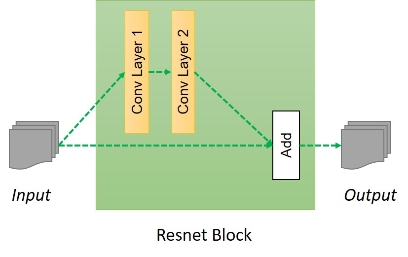
Code for Resnet block is as follow:
def resnet_blocks(input_res, num_features):

    out_res_1 = general_conv2d(input_res, num_features,
                               window_width=3,
                               window_heigth=3,
                               stride_width=1,
                               stride_heigth=1)
    out_res_2 = general_conv2d(out_res_1, num_features,
                               window_width=3,
                               window_heigth=3,
                               stride_width=1,
                               stride_heigth=1)
    return (out_res_2 + input_res)
Decoding
Up until now we have fed a feature vector $o_{enc}^{A}$ into a transformation layer to get another feature vector $o_{enc}^{B}$ of size $[64, 64, 256]$.
Decoding step is exact opposite of Step 1, we will build back the low level features back from the feature vector. This is done by applying a deconvolution (or transpose convolution) layer.
o_d1 = general_deconv2d(o_enc_B, num_features=ngf*2 window_width=3, window_height=3, stride_width=2, stride_height=2)
o_d2 = general_deconv2d(o_d1, num_features=ngf, window_width=3, window_height=3, stride_width=2, stride_height=2)
Finally we will convert this low level feature to image in domain $D_B$ as follow:
gen_B = general_conv2d(o_d2, num_features=3, window_width=7, window_height=7, stride_width=1, stride_height=1)
So, finally we have the generate image $gen_B$ of size $[256,256,3]$ and the code for building generator can be compressed to following function
def build_generator(input_gen):
    o_c1 = general_conv2d(input_gen, num_features=ngf, window_width=7, window_height=7, stride_width=1, stride_height=1)
    o_c2 = general_conv2d(o_c1, num_features=ngf*2, window_width=3, window_height=3, stride_width=2, stride_height=2)
    o_enc_A = general_conv2d(o_c2, num_features=ngf*4, window_width=3, window_height=3, stride_width=2, stride_height=2)

    # Transformation
    o_r1 = build_resnet_block(o_enc_A, num_features=64*4)
    o_r2 = build_resnet_block(o_r1, num_features=64*4)
    o_r3 = build_resnet_block(o_r2, num_features=64*4)
    o_r4 = build_resnet_block(o_r3, num_features=64*4)
    o_r5 = build_resnet_block(o_r4, num_features=64*4)
    o_enc_B = build_resnet_block(o_r5, num_features=64*4)

    #Decoding
    o_d1 = general_deconv2d(o_enc_B, num_features=ngf*2 window_width=3, window_height=3, stride_width=2, stride_height=2)
    o_d2 = general_deconv2d(o_d1, num_features=ngf, window_width=3, window_height=3, stride_width=2, stride_height=2)
    gen_B = general_conv2d(o_d2, num_features=3, window_width=7, window_height=7, stride_width=1, stride_height=1)

    return gen_B
Building the discriminator
We discussed how to build a generator, however for adversarial training of the network we need to build a discriminator as well. The discriminator would take an image as an input and try to predict if it is an original or the output from the generator. Generator can be visualized in following image.
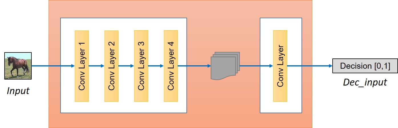
The discriminator is simply a convolution network in our case. First, we will extract the features from the image.
o_c1 = general_conv2d(input_disc, ndf, f, f, 2, 2)
o_c2 = general_conv2d(o_c1, ndf*2, f, f, 2, 2)
o_enc_A = general_conv2d(o_c2, ndf*4, f, f, 2, 2)
o_c4 = general_conv2d(o_enc_A, ndf*8, f, f, 2, 2)
Next step is deciding whether these features belongs to that particular category or not. For that we will add a final convolution layer that produces a 1 dimensional output. Here, $ndf$ denotes the number of features in initial layer of discriminator that one can vary or experiment with to get the best result.
decision = general_conv2d(o_c4, 1, f, f, 1, 1, 0.02)
We now have two main components of the model, namely Generator and Discriminator, and since we want to make this model work in both the direction i.e., from $A \rightarrow B$ and from $ B \rightarrow A$, we will have two Generators, namely $Generator_{A\rightarrow B}$ and $Generator_{B\rightarrow A}$, and two Discriminators, namely $Discriminator_A$ and $Discriminator_B$.
Building the model
Before getting to loss funtion let us define the base and see how to take input, construct the model.
input_A = tf.placeholder(tf.float32, [batch_size, img_width, img_height, img_layer], name="input_A")
input_B = tf.placeholder(tf.float32, [batch_size, img_width, img_height, img_layer], name="input_B")
These placeholders will act as input while defining our model as follow.
gen_B = build_generator(input_A, name="generator_AtoB")
gen_A = build_generator(input_B, name="generator_BtoA")
dec_A = build_discriminator(input_A, name="discriminator_A")
dec_B = build_discriminator(input_B, name="discriminator_B")

dec_gen_A = build_discriminator(gen_A, "discriminator_A")
dec_gen_B = build_discriminator(gen_B, "discriminator_B")
cyc_A = build_generator(gen_B, "generator_BtoA")
cyc_B = build_generator(gen_A, "generator_AtoB")
Above variable names are quite intuitive in nature. $gen$ represents image generated after using corresponding Generator and $dec$ represents decision after feeding the corresponding input to the discriminator.
Loss Function
By now we have two generators and two discriminators. We need to design the loss function in a way which accomplishes our goal. The loss function can be seen having four parts:
- Discriminator must approve all the original images of the corresponding categories.
- Discriminator must reject all the images which are generated by corresponding Generators to fool them.
- Generators must make the discriminators approve all the generated images, so as to fool them.
- The generated image must retain the property of original image, so if we generate a fake image using a generator say $Generator_{A\rightarrow B}$ then we must be able to get back to original image using the another generator $Generator_{B\rightarrow A}$ - it must satisfy cyclic-consistency.
D_A_loss_1 = tf.reduce_mean(tf.squared_difference(dec_A,1))
D_B_loss_1 = tf.reduce_mean(tf.squared_difference(dec_B,1))
Part 2
Since, discriniator should be able to distinguish between generated and original images, it should also be predicting 0 for images produced by the generator, i.e. Discriminator A wwould like to minimize $(Discriminator_A(Generator_{B\rightarrow A}(b)))^2$. It can be calculated as follow:
D_A_loss_2 = tf.reduce_mean(tf.square(dec_gen_A))
D_B_loss_2 = tf.reduce_mean(tf.square(dec_gen_B))

D_A_loss = (D_A_loss_1 + D_A_loss_2)/2
D_B_loss = (D_B_loss_1 + D_B_loss_2)/2
Generator loss
Generator should eventually be able to fool the discriminator about the authencity of it's generated images. This can done if the recommendation by discriminator for the generated images is as close to 1 as possible. So generator would like to minimize $(Discriminator_B(Generator_{A\rightarrow B}(a)) -1)^2$ So the loss is:
g_loss_B_1 = tf.reduce_mean(tf.squared_difference(dec_gen_A,1))
g_loss_A_1 = tf.reduce_mean(tf.squared_difference(dec_gen_A,1))
Cyclic loss
And the last one and one of the most important one is the cyclic loss that captures that we are able to get the image back using another generator and thus the difference between the original image and the cyclic image should be as small as possible.
cyc_loss = tf.reduce_mean(tf.abs(input_A-cyc_A)) + tf.reduce_mean(tf.abs(input_B-cyc_B))
The complete generator loss is then:
g_loss_A = g_loss_A_1 + 10*cyc_loss
g_loss_B = g_loss_B_1 + 10*cyc_loss
The multiplicative factor of 10 for cyc_loss assigns more importance to cyclic loss than the discrimination loss.
Putting it together
With the loss function defined, all the is needed to train the model is to minimize the loss function w.r.t. model parameters.
d_A_trainer = optimizer.minimize(d_loss_A, var_list=d_A_vars)
d_B_trainer = optimizer.minimize(d_loss_B, var_list=d_B_vars)
g_A_trainer = optimizer.minimize(g_loss_A, var_list=g_A_vars)
g_B_trainer = optimizer.minimize(g_loss_B, var_list=g_B_vars)
Training the model
for epoch in range(0,100):
    # Define the learning rate schedule. The learning rate is kept
    # constant upto 100 epochs and then slowly decayed
    if(epoch < 100) :
        curr_lr = 0.0002
    else:
        curr_lr = 0.0002 - 0.0002*(epoch-100)/100

    # Running the training loop for all batches
    for ptr in range(0,num_images):

        # Train generator G_A->B
        _, gen_B_temp = sess.run([g_A_trainer, gen_B],
                                 feed_dict={input_A:A_input[ptr], input_B:B_input[ptr], lr:curr_lr})

        # We need gen_B_temp because to calculate the error in training D_B
        _ = sess.run([d_B_trainer],
                     feed_dict={input_A:A_input[ptr], input_B:B_input[ptr], lr:curr_lr})

        # Same for G_B->A and D_A as follow
        _, gen_A_temp = sess.run([g_B_trainer, gen_A],
                                 feed_dict={input_A:A_input[ptr], input_B:B_input[ptr], lr:curr_lr})
        _ = sess.run([d_A_trainer],
                     feed_dict={input_A:A_input[ptr], input_B:B_input[ptr], lr:curr_lr})
You can see in above training function that one by one we are calling trainers corresponding to different Dicriminators and Generators. For training them, we need to feed traing images and learning rate of the optimizer. Since, we have batch_size = 1, so, num_batches = num_images.
Since, we are nearly done with the code, below is look at the default parameters that we took to train the model
Generated Image Pool
Calculating the discriminator loss for each generated image would be computationally prohibitive. To speed up training we store a collection of previously generated images for each domain and to use only one of these images for calculating the error. First, fill the image_pool one by one until its full and after that randomly replace an image from the pool and store the latest one and use the replaced image for training in that iteration.
def image_pool(self, num_gen, gen_img, gen_pool):
    if(num_gen < pool_size):
        gen_img_pool[num_gen] = gen_img
        return gen_img
    else :
        p = random.random()
        if p > 0.5:
            # Randomly selecting an id to return for calculating the discriminator loss
            random_id = random.randint(0,pool_size-1)
            temp = gen_img_pool[random_id]
            gen_pool[random_id] = gen_img
            return temp
        else :
            return gen_img
gen_image_pool_A = tf.placeholder(tf.float32, [batch_size, img_width, img_height, img_layer], name="gen_img_pool_A")
gen_image_pool_B = tf.placeholder(tf.float32, [batch_size, img_width, img_height, img_layer], name="gen_img_pool_B")

gen_pool_rec_A = build_gen_discriminator(gen_image_pool_A, "d_A")
gen_pool_rec_B = build_gen_discriminator(gen_image_pool_B, "d_B")

# Also the discriminator loss will change as follow

D_A_loss_2 = tf.reduce_mean(tf.square(gen_pool_rec_A))
D_A_loss_2 = tf.reduce_mean(tf.square(gen_pool_rec_A))
The image pool requires minor modifications to the code. For complete code refer to the implementation here.
Results
We ran the model for horse2zebra dataset but because of the lack of resources, we just ran the model for 100 epochs and got following results.
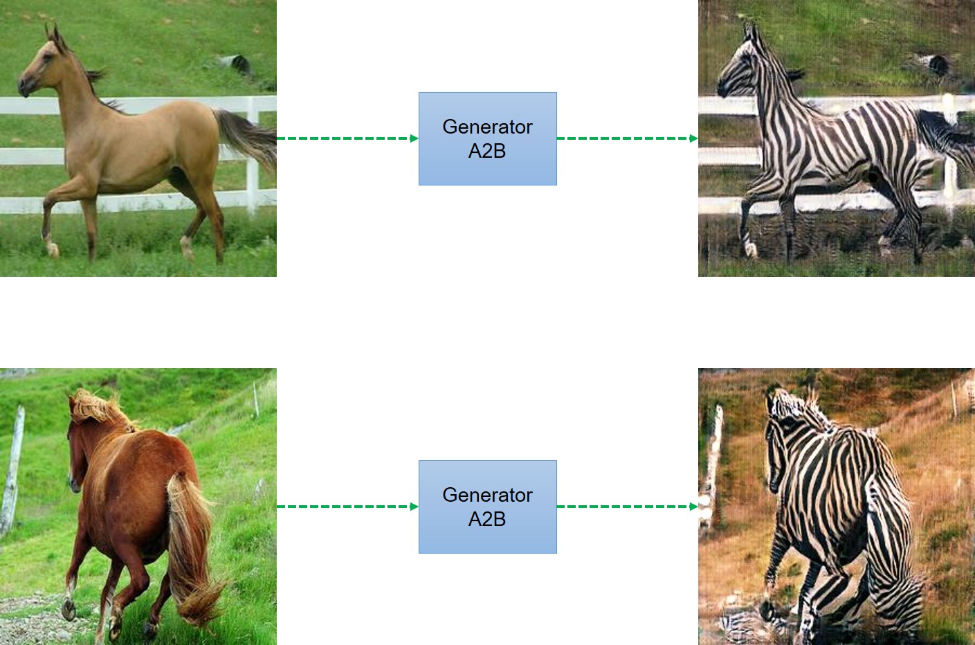
Results
Final Comments
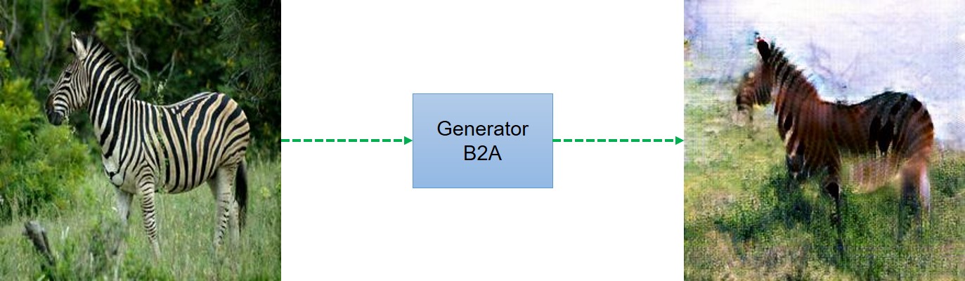
- During training we noticed that the ouput results were sensitive to initialization. Thanks to vanhuyz for pointing this out and suggesting training multiple times to get best results. You might notice background color being reversed as in following image. This effect can be observed only after 10-20 epochs and you can try to run the code again.
Distortion - We also think that this model is not good fit to change the shape of object. We tried to run the model for converting a men's face to a look alike women's face. For that we used celebA dataset but the results are not good and images produced are quite distorted.
If you spot any mistakes or feel if we missed anything please tell us about it in the comments. Thanks! for reading the blog.